2017年9月15日 星期五

[Python] 機器學習筆記 - 使用 準確率/召回率 (Precision-Recall) 評估分析成果

研究所時,算是第一次接觸這名詞,老闆的研究領域是 Search Engines ,用來評估索引成果好不好。最近則打算用在機器學習的成果分析,卻想不起當時老闆用來解釋索引成果的案例,還是容易忘記 XD 網路上打滾一下,發現這篇寫的廣告投放實際案例很好懂,也不容易忘,建議可以逛一下:準確率(Precision)與召回率(Recall)

回到本文,單純紀錄如何用既有函式庫計算:

import numpy as np
from sklearn.metrics import average_precision_score, precision_score, recall_score

# Classification metrics can't handle a mix of binary and continuous targets
#y = np.array([0, 0, 1, 1])
#scores = np.array([0.1, 0.3, 0.2, 0.8])

y = [0, 0, 1, 1]
scores = [0, 1, 1, 1]

#print(precision_score(y, scores, average='macro'))
#print(recall_score(y, scores, average='macro'))
#print(average_precision_score(y, scores))
#import sys
#sys.exit(0)

print('precision: %0.2f, recall: %0.2f, score: %0.2f' % (
        precision_score(y, scores, average='macro'),
        recall_score(y, scores, average='macro'),
        average_precision_score(y, scores)
))


成果:

precision: 0.83, recall: 0.75, score: 0.67

需要更詳細的範例,請參考:http://scikit-learn.org/stable/auto_examples/model_selection/plot_precision_recall.html

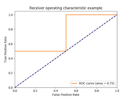
[Python] 機器學習筆記 - 使用 ROC 曲線 (receiver operating characteristic curve) 評估分析成果

roc curve

最近回想起兩年前走跳過的一場黑客松,當年的題目恰好是一個屬性的分類,就是一篇文章屬性給你,請告訴我它是不是 spam!所幸網路上還可以看到其他人的作品,逛了一下也順便研究別人的報告怎麼寫,其中有一組使用了 ROC 曲線來回報自己的分析成果,就來多多認識一下。

而 ROC 曲線是什麼?其實在 WIKI 或是 scikit-learn 文件(也引用WIKI資料)有很明確地解釋:
簡單的說,當畫出此圖後,若一開始就達左上角是最完美的,若一開始分析結果是斜線上方是好的,反之下方是差的。接下來,則是會去計算曲線下方的面積,產生一個介於 0~1 的數值,只要等於 0.5 就是跟隨機猜測一樣,代表此分析模型沒有預測價值;若大於 0.5 代表猜測是正向的,而小於 0.5 代表猜測的方向恰好相反;而 1 或 0 代表全部辨識正確或全部辨識錯誤。

因此,只需設法把模型預測結果畫一下 ROC 曲線,在算出個面積,就收工啦!

範例請參考 http://scikit-learn.org/stable/auto_examples/model_selection/plot_roc.html ,在此只筆記畫圖的部分:

import numpy as np
from sklearn.metrics import roc_curve, auc
y = np.array([0, 0, 1, 1])
scores = np.array([0.1, 0.4, 0.35, 0.8])
fpr, tpr, _ = roc_curve(y, scores)
roc_auc = auc(fpr, tpr)

import matplotlib as mpl
#mpl.use('Agg')
import matplotlib.pyplot as plt

fig = plt.figure()
lw = 2
plt.plot(fpr, tpr, color='darkorange', lw=lw, label='ROC curve (area = %0.2f)' % roc_auc)
plt.plot([0, 1], [0, 1], color='navy', lw=lw, linestyle='--')
plt.xlim([0.0, 1.0])
plt.ylim([0.0, 1.05])
plt.xlabel('False Positive Rate')
plt.ylabel('True Positive Rate')
plt.title('Receiver operating characteristic example')
plt.legend(loc="lower right")
#fig.savefig('/tmp/roc.png')
plt.show()

2017年9月14日 星期四

[MySQL] 從 JSON 抽取資料建立虛擬欄位 @ MySQL 5.7

同事反映 query 很慢,除了改進 SQL 語法外,也小試身手,對 JSON 資料抽出來建立虛擬欄位跟索引,順便筆記一下。

CREATE TABLE `my_data` (
  `id` int(11) unsigned NOT NULL AUTO_INCREMENT,
  `data` text,
  PRIMARY KEY (`id`),
) ENGINE=InnoDB DEFAULT CHARSET=utf8;


這邊 data column 是 text 型態,主因是這 DB server 從 5.6 升上來的 XD 且當初讓 data 有很多彈性,不一定是 json 格式。

但,要抽取成虛擬欄位時,建議要保持 data 是 json 格式,就先整理一下資料:

mysql> UPDATE my_data SET data = '{}' WHERE data IS NULL OR data = ''

假想 data 的數值為 {"keyword":"value"},因此抽出 keyword 虛擬欄位來用:

mysql> ALTER TABLE my_data ADD keyword VARCHAR(64) AS (JSON_UNQUOTE(data->>"$. keyword"));
mysql> ALTER TABLE my_data ADD INDEX (keyword);


如此一來,可以改對 keyword 欄位查詢了,可以再加快一點,而 table 狀態更新為:

CREATE TABLE `my_data ` (
  `id` int(11) unsigned NOT NULL AUTO_INCREMENT,
  `data` text,
  `keyword` varchar(64) GENERATED ALWAYS AS (json_unquote(json_unquote(json_extract(`data`,'$. keyword')))) VIRTUAL,
  PRIMARY KEY (`id`),
  KEY `keyword ` (`keyword `),
) ENGINE=InnoDB DEFAULT CHARSET=utf8;

2017年8月31日 星期四

[Python] 機器學習筆記 - sklearn.preprocessing 之 LabelEncoder, OneHotEncoder

最近挑一些資料來練習分析,想要用矩陣乘法,第一個念頭就是用 Hash table 把 keyword 轉成數值,接著要符合ㄧ些數學式子,又把數值擴展成 nx1 維,直到強者大大推坑看一些文件,我才發現這種招數很常使用,都有 library/framework 可以直接套用,順便把之前隨手寫的程式架構整理一下

先說一下 Hash table 的用法,就單純掃過所有數值,對所有數值建立查表方式,可以掃過一輪資料時,順便把標記都處理完畢:

import matplotlib.pyplot as plt
import seaborn as sns
import numpy as np

dataset = sns.load_dataset("tips")
print(dataset)
print(dataset.shape)
print(dataset.columns)
# Index(['total_bill', 'tip', 'sex', 'smoker', 'day', 'time', 'size'], dtype='object')

dataset_formated = None

# 土炮模式
fields_lookup = {}

print(dataset.columns)
for index, row in dataset.iterrows():
row_formated = np.empty([])

#for fieldname in dataset.columns:
for fieldname in [ 'day', 'smoker', 'time', 'sex', 'size' ]:
#print(field)

field_value = None
if fieldname not in fields_lookup:
fields_lookup[fieldname] = {}
if row[fieldname] not in fields_lookup[fieldname]:
fields_lookup[fieldname][ row[fieldname] ] = len(fields_lookup[fieldname])

# field value from hash table
field_data = np.zeros(1, dtype=np.int)
field_data[0] = fields_lookup[fieldname][ row[fieldname] ]

# handle row
row_formated = np.append( row_formated, field_data.reshape(1, -1) )

# handle data
if dataset_formated is None:
dataset_formated = np.zeros([ dataset.shape[0], row_formated.reshape(1, -1).size ], dtype=np.int)
dataset_formated[index] = row_formated.reshape(1, -1)
#print(row_formated)
#print(row_formated.reshape(1, -1))

print(fields_lookup)
print(dataset_formated)


如此一來就完成編碼,也完成資料格式轉換:

{'day': {'Sun': 0, 'Sat': 1, 'Thur': 2, 'Fri': 3}, 'smoker': {'No': 0, 'Yes': 1}, 'time': {'Dinner': 0, 'Lunch': 1}, 'sex': {'Female': 0, 'Male': 1}, 'size': {2: 0, 3: 1, 4: 2, 1: 3, 6: 4, 5: 5}}

然而,對於部分演算法可能拿編碼的整數進行運算,或是想要更精準把整數擴展成選擇結果,那解法就是擴展欄位,例如有 5 種結果,就擴展成 5 個欄位,選到的標 1 ,沒選到標 0,土炮處理方式就麻煩了點,需要先掃一次建立 hash table,接著第二次在重建數據:

# build hash table only
for index, row in dataset.iterrows():
#for fieldname in dataset.columns:
for fieldname in [ 'day', 'smoker', 'time', 'sex', 'size' ]:
#print(field)
if fieldname not in fields_lookup:
fields_lookup[fieldname] = {}
if row[fieldname] not in fields_lookup[fieldname]:
fields_lookup[fieldname][ row[fieldname] ] = len(fields_lookup[fieldname])

print(fields_lookup)

# build new matrix
for index, row in dataset.iterrows():
row_formated = np.empty([])

for fieldname in [ 'day', 'smoker', 'time', 'sex', 'size' ]:
# field value from hash table
field_data = np.zeros([len(fields_lookup[fieldname]), 1], dtype=np.int)
field_data[ fields_lookup[fieldname][row[fieldname]] ][0] = 1

# handle row
row_formated = np.append( row_formated, field_data.reshape(1, -1) )

#print(row_formated)

# handle data
if dataset_formated is None:
dataset_formated = np.zeros([ dataset.shape[0], row_formated.reshape(1, -1).size ], dtype=np.int)
dataset_formated[index] = row_formated.reshape(1, -1)
#print(row_formated)
#print(row_formated.reshape(1, -1))

print(dataset_formated)


回到常用的方式 - LabelEncoder:

from sklearn.preprocessing import LabelEncoder
from sklearn.preprocessing import OneHotEncoder

dataset_encode = dataset.copy()
labels = {}

for i, field in enumerate(dataset.columns):
if field == 'tip' or field == 'total_bill':
continue
labels[field] = list(set(dataset[field].unique()))
label_encoder = LabelEncoder()
label_encoder.fit(labels[field])

# original
#print(dataset_encode.iloc[:,i])
#print(dataset_encode[field])

# encode
#feature = label_encoder.transform(dataset_encode.iloc[:,i])
#feature = feature.reshape(dataset.shape[0], 1)
# https://stackoverflow.com/questions/24458645/label-encoding-across-multiple-columns-in-scikit-learn
dataset_encode[field] = label_encoder.fit_transform(dataset_encode[field])

#print(dataset_encode[field])

print(dataset_encode)


輸出:

     total_bill   tip  sex  smoker  day  time  size
0         16.99  1.01    0       0    2     0     1
1         10.34  1.66    1       0    2     0     2
2         21.01  3.50    1       0    2     0     2
3         23.68  3.31    1       0    2     0     1
4         24.59  3.61    0       0    2     0     3
5         25.29  4.71    1       0    2     0     3
6          8.77  2.00    1       0    2     0     1
7         26.88  3.12    1       0    2     0     3
8         15.04  1.96    1       0    2     0     1
9         14.78  3.23    1       0    2     0     1
10        10.27  1.71    1       0    2     0     1
11        35.26  5.00    0       0    2     0     3
12        15.42  1.57    1       0    2     0     1
13        18.43  3.00    1       0    2     0     3
14        14.83  3.02    0       0    2     0     1
15        21.58  3.92    1       0    2     0     1
16        10.33  1.67    0       0    2     0     2
17        16.29  3.71    1       0    2     0     2
18        16.97  3.50    0       0    2     0     2
19        20.65  3.35    1       0    1     0     2
20        17.92  4.08    1       0    1     0     1
21        20.29  2.75    0       0    1     0     1
22        15.77  2.23    0       0    1     0     1
23        39.42  7.58    1       0    1     0     3
24        19.82  3.18    1       0    1     0     1
25        17.81  2.34    1       0    1     0     3
26        13.37  2.00    1       0    1     0     1
27        12.69  2.00    1       0    1     0     1
28        21.70  4.30    1       0    1     0     1
29        19.65  3.00    0       0    1     0     1
..          ...   ...  ...     ...  ...   ...   ...
214       28.17  6.50    0       1    1     0     2
215       12.90  1.10    0       1    1     0     1
216       28.15  3.00    1       1    1     0     4
217       11.59  1.50    1       1    1     0     1
218        7.74  1.44    1       1    1     0     1
219       30.14  3.09    0       1    1     0     3
220       12.16  2.20    1       1    0     1     1
221       13.42  3.48    0       1    0     1     1
222        8.58  1.92    1       1    0     1     0
223       15.98  3.00    0       0    0     1     2
224       13.42  1.58    1       1    0     1     1
225       16.27  2.50    0       1    0     1     1
226       10.09  2.00    0       1    0     1     1
227       20.45  3.00    1       0    1     0     3
228       13.28  2.72    1       0    1     0     1
229       22.12  2.88    0       1    1     0     1
230       24.01  2.00    1       1    1     0     3
231       15.69  3.00    1       1    1     0     2
232       11.61  3.39    1       0    1     0     1
233       10.77  1.47    1       0    1     0     1
234       15.53  3.00    1       1    1     0     1
235       10.07  1.25    1       0    1     0     1
236       12.60  1.00    1       1    1     0     1
237       32.83  1.17    1       1    1     0     1
238       35.83  4.67    0       0    1     0     2
239       29.03  5.92    1       0    1     0     2
240       27.18  2.00    0       1    1     0     1
241       22.67  2.00    1       1    1     0     1
242       17.82  1.75    1       0    1     0     1
243       18.78  3.00    0       0    3     0     1

[244 rows x 7 columns]


若想保留之前的欄位,也可用添加新欄位的方式:

dataset_encode[field+"-encode"] = label_encoder.fit_transform(dataset_encode[field])

而 OneHotEncoder 則是因為產出的維度會變大,要再設法把新產出來的數值再添加回去:

from sklearn.preprocessing import LabelEncoder
from sklearn.preprocessing import OneHotEncoder

dataset_encode = dataset.copy()
labels = {}

for i, field in enumerate(dataset.columns):
if field == 'tip' or field == 'total_bill':
continue

# original
#print(dataset_encode.iloc[:,i])
#print(dataset_encode[field])

# LabelEncode
labels[field] = list(set(dataset[field].unique()))
label_encoder = LabelEncoder()
label_encoder.fit(labels[field])

# https://stackoverflow.com/questions/24458645/label-encoding-across-multiple-columns-in-scikit-learn
dataset_encode[field+"-LabelEncode"] = label_encoder.fit_transform(dataset_encode[field])
#dataset_encode[field] = label_encoder.fit_transform(dataset_encode[field])

# OneHotEncode
feature = label_encoder.transform(dataset_encode[field])
feature = feature.reshape(dataset.shape[0], 1)
# http://scikit-learn.org/stable/modules/generated/sklearn.preprocessing.OneHotEncoder.html
onehot_encoder = OneHotEncoder(sparse=False,n_values=len(labels[field]))
onehot_result = onehot_encoder.fit_transform(feature)
#dataset_encode[field+"-OneHotEncode"] = onehot_encoder.fit_transform(feature)
#onehot_encoder[ ["A","B"] ] = onehot_result

for index in range(len(labels[field])):
dataset_encode[field+"-OneHotEncode-"+str(index)] = onehot_result[:,index]

#print(dataset_encode[field])

print(dataset_encode.head(5))


如此一來,結果會是這樣:

   total_bill   tip     sex smoker  day    time  size  sex-LabelEncode  \
0       16.99  1.01  Female     No  Sun  Dinner     2                0
1       10.34  1.66    Male     No  Sun  Dinner     3                1
2       21.01  3.50    Male     No  Sun  Dinner     3                1
3       23.68  3.31    Male     No  Sun  Dinner     2                1
4       24.59  3.61  Female     No  Sun  Dinner     4                0

   sex-OneHotEncode-0  sex-OneHotEncode-1         ...           \
0                 1.0                 0.0         ...          
1                 0.0                 1.0         ...          
2                 0.0                 1.0         ...          
3                 0.0                 1.0         ...          
4                 1.0                 0.0         ...          

   time-LabelEncode  time-OneHotEncode-0  time-OneHotEncode-1  \
0                 0                  1.0                  0.0
1                 0                  1.0                  0.0
2                 0                  1.0                  0.0
3                 0                  1.0                  0.0
4                 0                  1.0                  0.0

   size-LabelEncode  size-OneHotEncode-0  size-OneHotEncode-1  \
0                 1                  0.0                  1.0
1                 2                  0.0                  0.0
2                 2                  0.0                  0.0
3                 1                  0.0                  1.0
4                 3                  0.0                  0.0

   size-OneHotEncode-2  size-OneHotEncode-3  size-OneHotEncode-4  \
0                  0.0                  0.0                  0.0
1                  1.0                  0.0                  0.0
2                  1.0                  0.0                  0.0
3                  0.0                  0.0                  0.0
4                  0.0                  1.0                  0.0

   size-OneHotEncode-5
0                  0.0
1                  0.0
2                  0.0
3                  0.0
4                  0.0

2017年8月29日 星期二

[Python] 機器學習筆記 - 使用 seaborn 呈現資料狀態(數據視覺化)

這陣子被高手推坑 kaggle ,越看越有動力,就順勢把很久以前欠的知識技術順勢補一下:資料視覺化。

在數據分析的比賽,默認的資料多是 csv 格式,接著用 panda 讀取,再用 seaborn 和 matplotlib.pyplot 繪圖。透過第一步的視覺化,快速得知數據分佈狀態,甚至在

輸入資料:

     total_bill   tip     sex smoker   day    time  size
0         16.99  1.01  Female     No   Sun  Dinner     2
1         10.34  1.66    Male     No   Sun  Dinner     3
2         21.01  3.50    Male     No   Sun  Dinner     3
3         23.68  3.31    Male     No   Sun  Dinner     2
4         24.59  3.61  Female     No   Sun  Dinner     4
5         25.29  4.71    Male     No   Sun  Dinner     4
6          8.77  2.00    Male     No   Sun  Dinner     2
7         26.88  3.12    Male     No   Sun  Dinner     4
8         15.04  1.96    Male     No   Sun  Dinner     2
9         14.78  3.23    Male     No   Sun  Dinner     2
10        10.27  1.71    Male     No   Sun  Dinner     2
11        35.26  5.00  Female     No   Sun  Dinner     4
12        15.42  1.57    Male     No   Sun  Dinner     2
13        18.43  3.00    Male     No   Sun  Dinner     4
14        14.83  3.02  Female     No   Sun  Dinner     2
15        21.58  3.92    Male     No   Sun  Dinner     2
16        10.33  1.67  Female     No   Sun  Dinner     3
17        16.29  3.71    Male     No   Sun  Dinner     3
18        16.97  3.50  Female     No   Sun  Dinner     3
19        20.65  3.35    Male     No   Sat  Dinner     3
20        17.92  4.08    Male     No   Sat  Dinner     2
21        20.29  2.75  Female     No   Sat  Dinner     2
22        15.77  2.23  Female     No   Sat  Dinner     2
23        39.42  7.58    Male     No   Sat  Dinner     4
24        19.82  3.18    Male     No   Sat  Dinner     2
25        17.81  2.34    Male     No   Sat  Dinner     4
26        13.37  2.00    Male     No   Sat  Dinner     2
27        12.69  2.00    Male     No   Sat  Dinner     2
28        21.70  4.30    Male     No   Sat  Dinner     2
29        19.65  3.00  Female     No   Sat  Dinner     2
..          ...   ...     ...    ...   ...     ...   ...
214       28.17  6.50  Female    Yes   Sat  Dinner     3
215       12.90  1.10  Female    Yes   Sat  Dinner     2
216       28.15  3.00    Male    Yes   Sat  Dinner     5
217       11.59  1.50    Male    Yes   Sat  Dinner     2
218        7.74  1.44    Male    Yes   Sat  Dinner     2
219       30.14  3.09  Female    Yes   Sat  Dinner     4
220       12.16  2.20    Male    Yes   Fri   Lunch     2
221       13.42  3.48  Female    Yes   Fri   Lunch     2
222        8.58  1.92    Male    Yes   Fri   Lunch     1
223       15.98  3.00  Female     No   Fri   Lunch     3
224       13.42  1.58    Male    Yes   Fri   Lunch     2
225       16.27  2.50  Female    Yes   Fri   Lunch     2
226       10.09  2.00  Female    Yes   Fri   Lunch     2
227       20.45  3.00    Male     No   Sat  Dinner     4
228       13.28  2.72    Male     No   Sat  Dinner     2
229       22.12  2.88  Female    Yes   Sat  Dinner     2
230       24.01  2.00    Male    Yes   Sat  Dinner     4
231       15.69  3.00    Male    Yes   Sat  Dinner     3
232       11.61  3.39    Male     No   Sat  Dinner     2
233       10.77  1.47    Male     No   Sat  Dinner     2
234       15.53  3.00    Male    Yes   Sat  Dinner     2
235       10.07  1.25    Male     No   Sat  Dinner     2
236       12.60  1.00    Male    Yes   Sat  Dinner     2
237       32.83  1.17    Male    Yes   Sat  Dinner     2
238       35.83  4.67  Female     No   Sat  Dinner     3
239       29.03  5.92    Male     No   Sat  Dinner     3
240       27.18  2.00  Female    Yes   Sat  Dinner     2
241       22.67  2.00    Male    Yes   Sat  Dinner     2
242       17.82  1.75    Male     No   Sat  Dinner     2
243       18.78  3.00  Female     No  Thur  Dinner     2

[244 rows x 7 columns]


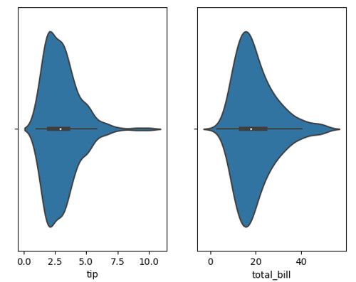
繪出資料分佈/密布圖:

sns1

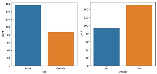
繪出資料筆數:

sns2

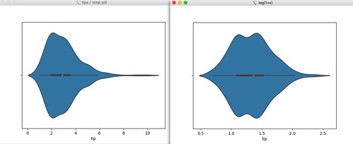
繪出 log(1+x) 的效果(以 tip 為例):

sns3

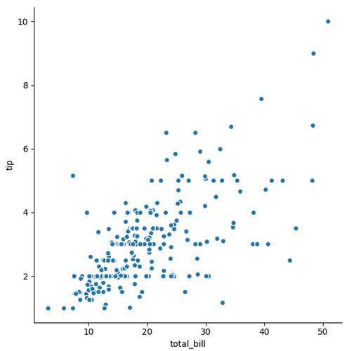
兩兩欄位計算相關性,並繪出分佈圖:

sns4

程式碼:

import matplotlib.pyplot as plt
import seaborn as sns

tips = sns.load_dataset("tips")
print(tips)

# https://seaborn.pydata.org/generated/seaborn.violinplot.html
plt.figure('tips / total_bill')
plt.subplot(1,2,1)
sns.violinplot(data=tips, x='tip')

plt.subplot(1,2,2)
sns.violinplot(data=tips, x='total_bill')

# https://seaborn.pydata.org/generated/seaborn.countplot.html
plt.figure('sex / smoker')
plt.subplot(1,2,1)
sns.countplot(data=tips,x='sex')
plt.subplot(1,2,2)
sns.countplot(data=tips,x='smoker')

import numpy as np

plt.figure('log(1+x)')

# https://docs.scipy.org/doc/numpy/reference/generated/numpy.log1p.html
tips['tip'] = np.log1p(tips['tip'])
sns.violinplot(data=tips, x='tip')

# https://pandas.pydata.org/pandas-docs/stable/generated/pandas.DataFrame.corr.html
data_corr = tips.corr()
print(data_corr)

threshold = 0.5
corr_list = []
size = data_corr.shape[0]
for i in range(0,size):
for j in range(i+1,size):
if (data_corr.iloc[i,j] >= threshold and data_corr.iloc[i,j] < 1) or (data_corr.iloc[i,j] < 0 and data_corr.iloc[i,j] <= -threshold):
corr_list.append([data_corr.iloc[i,j],i,j])

s_corr_list = sorted(corr_list,key=lambda x: -abs(x[0]))
print(s_corr_list)

cols=data_corr.columns
for v,i,j in s_corr_list:
print ("%s and %s = %.2f" % (cols[i],cols[j],v))
sns.pairplot(tips, size=6, x_vars=cols[i],y_vars=cols[j] )

plt.show()


最後,有時資料內有垃圾需要清除後在繪圖,可以善用 pandas.DataFrame.dropna 來過濾資料:

# https://pandas.pydata.org/pandas-docs/stable/generated/pandas.DataFrame.dropna.html
# 繪圖時,刪除 nan 的資料
newdata = rawdata.dropna(axis=0)
sns.violinplot(newdata)

# https://pandas.pydata.org/pandas-docs/stable/generated/pandas.DataFrame.drop.html
# 繪圖時,只關注特定範圍的資料(此例:總額 < 20 都刪除不繪)

newdata = tips.drop(tips[ tips.total_bill < 20 ].index)
sns.violinplot(data=newdata, x='tip')